Understanding Solve Time in MIP Supply Chain Models Using Community Data

For network models run through Coupa's supply chain modeling application, Supply Chain Modeler, we’re often asked how long a scenario will take to run or how to decrease its solve time in future runs. Historically, this has been a hard question to answer. The underlying engine (a mixed integer program, or MIP) is known to be part of a class of algorithms where there’s serious doubt if there will ever be a guaranteed way to solve the models quickly.

Applying community data to supply chain modeling

We turned to the community data we have to help answer this question. For each cloud model run via Coupa Supply Chain Modeler, the anonymous model and solution log information are pulled into a central database. This provides the exact counts of every variable included in each supply chain model run through the service, as well as the relative solution path the solver took to optimize the network problem. We currently have ~60,000 model runs and their relative features in our current dataset. These have been collected across our community of users, spanning most industries with physical supply chains. This process continues today with over 1,000 new models being recorded weekly.

We’re now starting to use this data to help our customers understand their models — and, more specifically, what drives the complexity and solve time. To give you a sense of the data, the median size for these 60,000 models is:

• Number of Sites: 312
• Number of Customers: 200
• Number of Demand Records: 1811
• Number of Products: 28
• Number of Time Periods: 1

This shows that the median supply chain model our customer base is solving is relatively small. However, many customers are pushing the solver limits. If we look at the largest 8,000 models in our dataset, the medians are a lot larger:

• Number of Sites: 980
• Number of Customers: 714
• Number of Demand Records: 222,761
• Number of Products: 1,268
• Number of Time Periods: 12

If we look at the run times, most of the 60,000 supply chain models run are less than 5 minutes. However, there are still a significant number of models that took much longer. Here’s the distribution of run time across the models in the dataset:

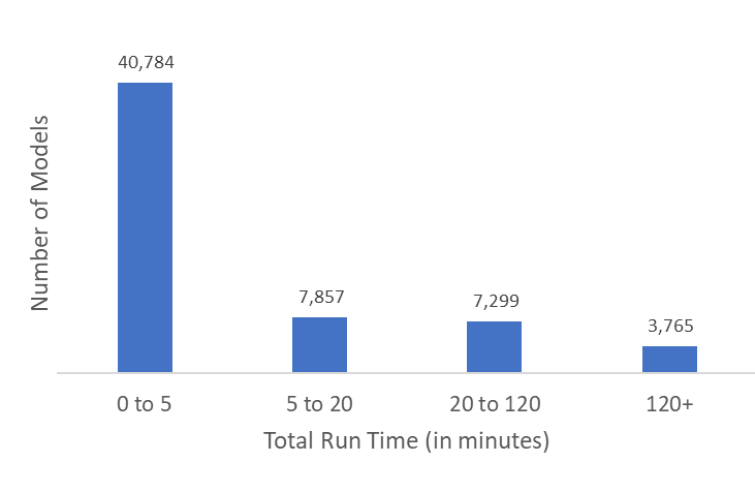
But this data doesn’t tell the whole story. When it comes to supply chain modeling, we can assume the number of desired long-running models is significantly more than the ones that were actually run. If a model takes a long time to run, our users likely won’t run it as often as they might otherwise, or they may not test as many scenarios, driving the number of data points in the longer time buckets down. To add to the effect, often users may only run the model once, scaling it down after to avoid the complexity all together.

Therefore, it’s still important that we understand the long run times so more customers can create and run the large models if they want or require that level of detail.

Predicting run times with supply chain modeling

Over the years, multiple attempts at predicting network model run time have been made with little to no success. However, those studies largely focused on leveraging the number of continuous variables and/or integer variables in the supply chain models relative to the solve time. In the charts below, we’ve zoomed in on a subset of the models. There’s a very slight trend that bigger models take longer to run — but you can see that for any model size, there’s a huge variation of run times.

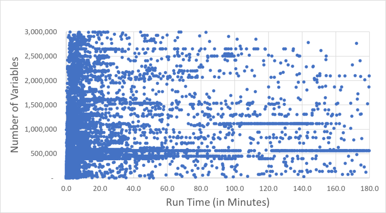
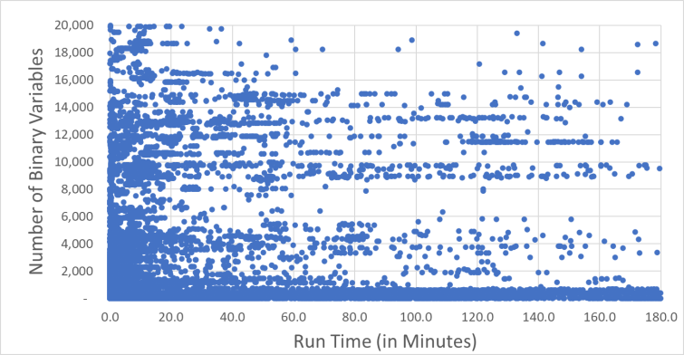
Thus, predicting run time based on variables or binary variables alone is extremely inaccurate due to the concentration of models around low solve times regardless of variable count. Further, looking at supply chain models with longer run times, historical data yields some with small and others with large counts of variables also contributing to the concern. Users are left with no idea of run time until they run through the solve and no real idea for how to reduce those run times.

Leveraging community data in supply chain modeling

As mentioned, previous studies struggled to find predictability as they only considered the primary variable counts of the supply chain models. They did this because their models consisted of all kinds of MIPs with significantly different formulations and/or didn’t have access to an appropriate dataset. In our community, we’re all solving a similar problem leveraging the same base formulation across all models. Therefore, each model in the dataset contains a subset of over 300 specific model variables and constraints, each model being a unique configuration of those same features. The obvious question emerged of whether to leverage them instead to predict the run time. We know not all variables are created equal — the real question is which ones are driving the run time more significantly.

When we expanded the study to include each of those 300 model features and their relative counts, predictability began to show. Over several iterations of improving the predictive supply chain modeling and comparing several different predictive algorithms, the XGBoost machine learning (ML)-based algorithm emerged as the clear winner. XGBoost is an algorithm that has seen recent attention in the area of applied ML, which is based on an implementation of gradient-boosted decision trees designed for speed and performance.

Initial predictive models were set to predict low complexity/fast network models first, looking at predicting solve time at the five-minute mark. From there, several child models were developed to classify run time into three additional buckets: from 5–20 minutes, from 20–120 minutes, and above 120 minutes. Our accuracy was highest for the 0–5-minute bucket at 96% precision (the recall was the same 96%, and all our results showed recall was nearly the same as precision, so we’ll report on just precision). The other buckets ranged from 81% to 88% accuracy.

We felt the results were accurate enough to get valuable information. As important as the prediction, this same XGBoost based method surfaces specific features and their relative weights that contribute most to the predictions. On average, the features shown in the chart below contribute most to a model’s complexity. For each specific run, different combinations of features and relative weights can help to identify specific areas to that supply chain model that can be reduced for more precise model adjustments. Recent improvements to the classification process have helped to better understand the relative weights, and how they can be translated into an actual magnitude of change for the model to be classified in the next lower level.

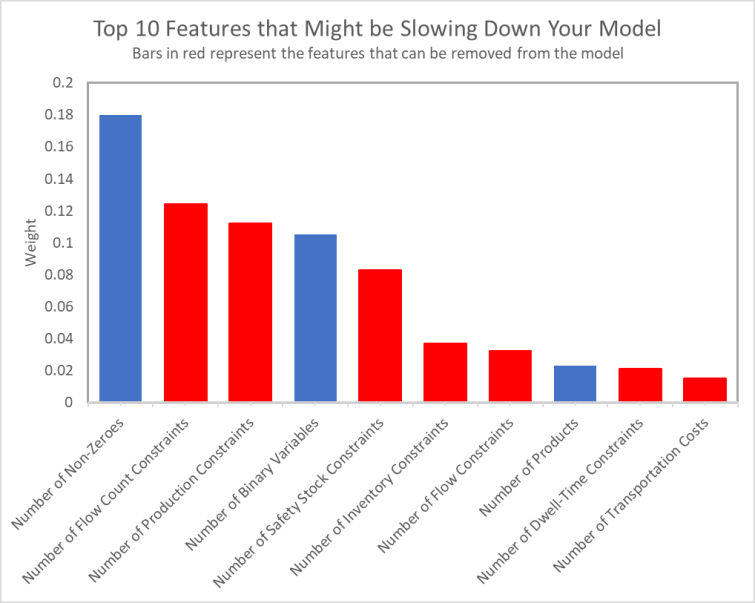
From these averages, we still see the trend that bigger supply chain models are generally more complicated. When this is the primary driver for run time — and in other cases where the prediction indicates a model that’s too large — aggregating, splitting, and/or trimming the model may be necessary to get it down to a more practical level. However, when looking at the other primary drivers, we also see specific model features emerging as the primary driver for run time in many cases. Often, it’s the number of elements within a single constraint or cost type that’s causing the model to underperform. Either way, knowing what’s driving the complexity is a first step towards resolving it. For each of the top 10 features, here’s a quick run-down of what they really mean, and some prescriptions for mitigation:    

1. Number of Non-Zeros: This would indicate the model is likely too large across multiple dimensions. Removing costs, constraints, and timing from the model can help; otherwise scaling down the model across multiple elements is recommended. 
2. Number of Flow Count Constraints: The model has too many restrictions relating to number of possible lane combinations where enumerating them creates too large of a solution space. Removing constraints that aren’t binding on the expected model result can help to reduce this without having a significant effect on the model accuracy.
3. Number Production Throughput Constraints: The model has too many restrictions on production capacity, often causing the feasible solution space to become small. Users can consider removing non-binding constraints or adjusting constraint granularity to help increase solvability.
4. Number of Binary Variables: The number of binary variables is leading to scaling issues due to enumeration of possible variable combinations. Consider removing binaries that have a small effect on the solution, or consider splitting the model to reduce the possible combinations.
5. Number of Safety Stock Constraints: This indicates the model has too many restrictions on inventory levels, often leading to misalignment between needed supply and end demand in the model. Removing constraints that are non-binding or aggregating constraints can help reduce the model complexity and feasibility. 
6. Number of Inventory Variables: Inventory variables are primarily used to connect activity between periods in our formulation. When there are too many, reducing the number of site-product-period combinations in the model, or removing inventory capabilities from sites that aren’t storage locations, can drive the number down.
7. Number of Flow Constraints: This is similar to production constraints but on the lane side, likely leading to a situation where the feasible solution space becomes too small. Similarly, removing non-binding constraints or aggregating constraints can help to reduce this complexity.
8. Number of Products: When products are too many, it’s likely an indication that the model is a bit too big as well. Aggregating or removing insignificant products from the model are likely the best ways to increase model performance.
9. Number of Dwell Time Constraints: These constraints have similar consequences, as inventory variables in the model and control how long a product can stay at a particular location. Removing limits that are non-binding and/or leveraging a multi-objective approach can help to keep the effect without losing significant accuracy.
10. Number of Transportation Costs: This is likely related to the number of lanes or source destination combinations in the model. Removing insignificant costs or trimming the model to not include source combinations that are unlikely can have a good effect on this feature count.

Endless supply chain modeling possibilities going forward

This analysis has proven that predicting run time of MIP-based supply chain network models is possible when considering models sharing the same base formulation given enough detail into the model features. Improvements to the predictive model based on including more model info, like statistical detail around the variables themselves, are expected to further improve the future accuracy of the model.

Additionally, new initiatives are kicking off that look to leverage the data and prediction itself in more creative ways. Imagine a world where a model could auto correct itself to become more solvable, or could have a guiding hand when building models based on alignment with other network models in the community. Keep an eye out for new features in the upcoming Coupa Supply Chain Design & Planning releases that look to transform supply chain design as we begin to integrate more advanced AI-based concepts directly into the modeling process.